CS 7641 - Acoustify, Group 3 Spring 2021

Link to final presentation video

https://musicclassification.github.io/

Members (Group 3 on Canvas)

Sidhesh Desai, Pranay Agrawal, Ayush Nene, Manoj Niverthi, Pranal Madria

Overview

In this project, we aim to use supervised and unsupervised learning for music classification purposes.

Introduction

As avid music listeners, we so often find ourselves listening to the same genres and types of music on a consistent basis. Creating a tool that would allow music enthusiasts to discover, curate, share, and compare pieces of music would allow listeners to foray into a whole new musical experience – one that would drastically improve the diversity of musical tracks they listen to. As such, we aim to create a music classification tool to allow for the grouping together of similar types of music based on acoustic and non-acoustic features as well as the recognition of music genre from a given piece of music. Through this project, we were successfully able to do so.

Problem Definition

Given a piece of music, we would like to use a supervised approach to accurately classify the genre to which it belongs. For the unsupervised approach, we aim to group the music with other similar types of music based on both acoustic and non-acoustic features and provide recommendations for other songs which are similar to the sample in question.

Data Collection

We began by looking for datasets involving music. As stated in our project proposal, we found the datasets GTZAN and Million Songs as the perfect match. We started by downloading these datasets and we began by using the 30-second songs feature dataset. We wanted to see correlations between features and thus we used a heatmap to visually identify correlations between different features.

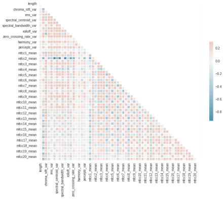
As seen, certain features were highly correlated with others. Thus, this inspired us to transform our data from 58 features to 2 engineered features using PCA as this will simplify our dataset while withholding important information.

Here, we will explain some of the features within this dataset: Zero Crossing Rate: the rate at which the the audio signal modulates between positive and negative Mel-Frequency Cepstral Coefficients (MFCC): a set of features which essentially capture the human envelope of speech (in the dataset, we use 20 of these features) Spectral Centroid: the weighted average of frequencies samples at a specific point in time Spectral Rolloff: shape of the signal that represents a threshold below which most of the signal lies Tempo BPM: beats per minute in the audio piece Harmonics: overtones which are present in the sound sample (very hard to distinguish using the human ear) Perceptual: features that encodes the rhythm and beat of the piece

Methods

The first step will involve constructing a music dataset and extracting features about different songs – both acoustic features and non-acoustic features. From that point onward, we will separate our analysis into two parts – an unsupervised component and a supervised component. We will use supervised learning to predict the genre of a piece of music, comparing the performance of models such as Support Vector Machines, K-Nearest Neighbors, and Naive Bayes. We can employ unsupervised learning to cluster the dataset based on acoustic and non-acoustic features. These clusters can be used to give suggestions for other songs that the user may enjoy. These models will be trained and tested using the GTZAN and Million Song datasets, and we will use grid search in order to fine-tune our hyperparameters. Employing principal component analysis will allow us to reduce the dimensionality of our dataset.

Unsupervised

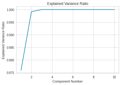
The original dataset had 58 features and thus we decided to transform our dataset using PCA. We wanted to determine the optimal number of principal components, thus we used the explained variance ratio.

PCA

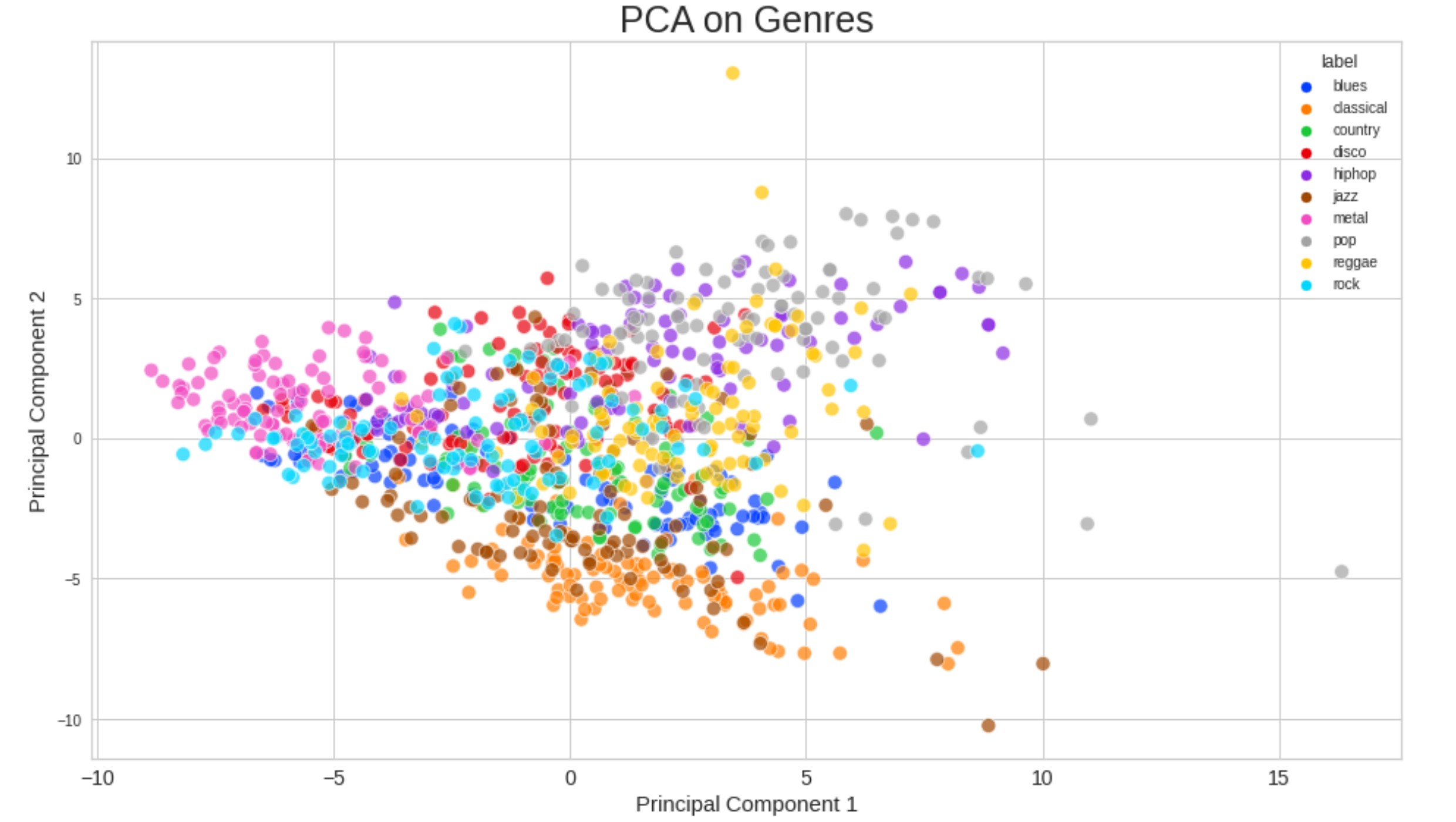
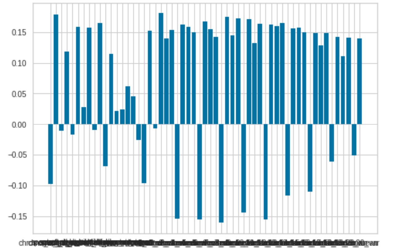
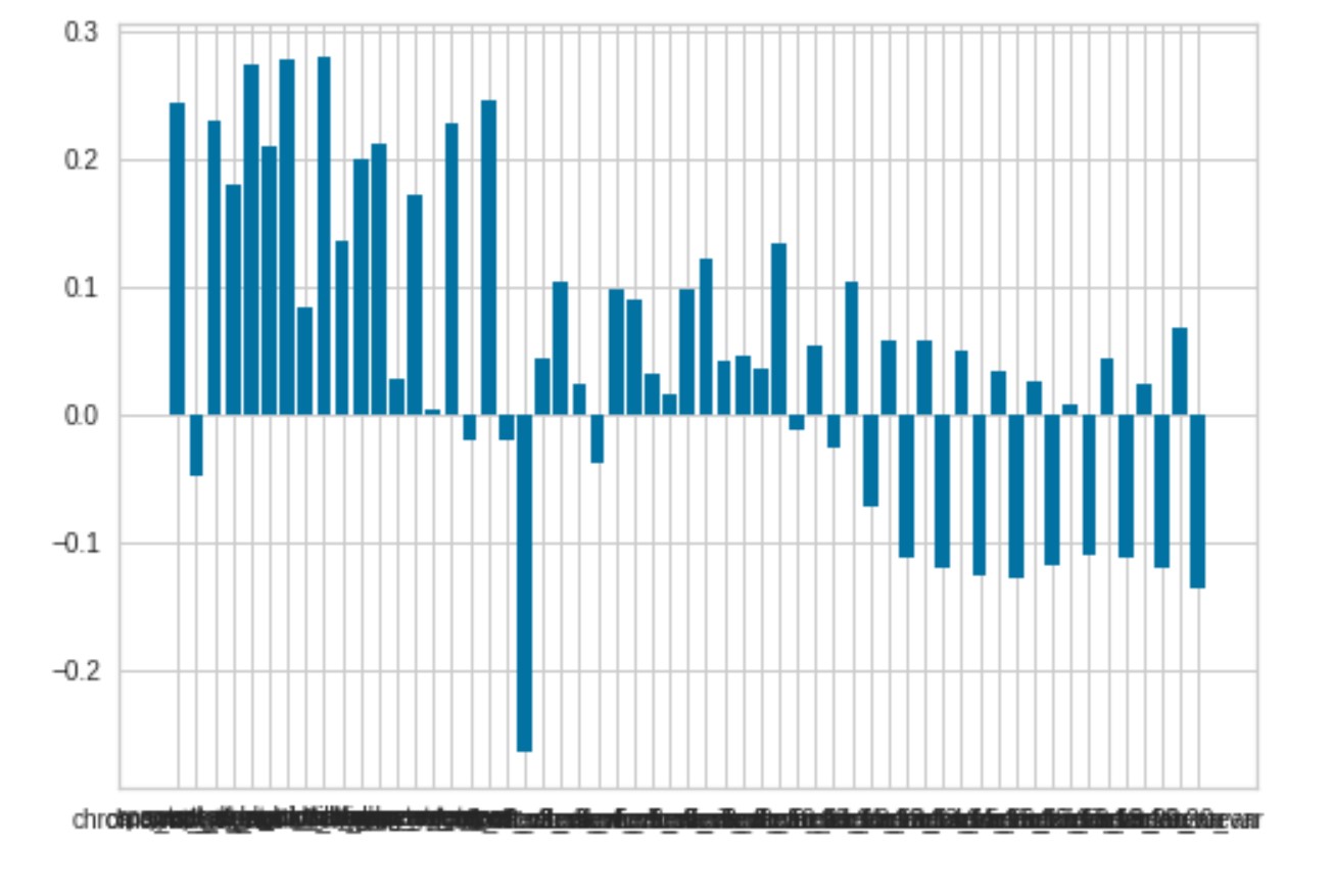
As we can see, it appears that the first principal component mainly consists of 3 of the original features, while the second principal component mainly consists of 4 of the original features. We will partition the array to figure out which ones these are.

We can see that running PCA on our dataset provides a greatly simplified feature set that is still able to capture the vast majority of variance present in the dataset. With just num_features=2, we are able to capture > 0.99 of the variance in the original dataset, prompting us to utilize this as our threshold value for our features post-PCA.

Thus, we successfully transformed our original dataset of 58 features into a simplified feature set of just 2 engineered features. We wanted to use both the transformed and pre-transformed data when employing our approaches for exploratory reasons as we could compare the two feature sets.

Now, we were ready to begin employing our unsupervised/supervised learning approaches.

We began by employing unsupervised learning where we used GMM and K-Means to cluster our data. For K-Means, we used the elbow method to determine the optimal number of clusters : For the pre-transformed data (with 58 features) we received this when utilizing the elbow method:

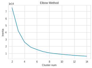
As seen, the optimal number of clusters determined by the elbow method was 5.

For the transformed data post PCA, the output was as follows:

As seen, the post PCA data which had 2 engineered features, was extremely similar to the first when utilizing the elbow method. The optimal number of clusters, as determined by the elbow method, was 5.

We then ran K-Means with 5 clusters and the output and analysis is listed in the results section.

Afterwards, we utilized our other clustering method: GMM. For GMM, we clustered the data using several different numbers of clusters and then used the silhouette coefficient to analyze the optimal number of clusters as well as the purity scores to evaluate the quality of clustering. The outputs are in the Results section.

Custom Genres

Further for the unsupervised portion, we also added custom genres which were combinations of genres. We will attempt to apply prior knowledge in order to group genres by how similar we believe they are. Then we will apply our supervised learning to these supergenres to see if it will improve the accuracy.

The supergenres we will use are as follows, based on our initial K-Means clustering:

1. classical, jazz
2. pop, hiphop
3. country, blues
4. metal
5. rock, disco
6. reggae

We also tried K-means clustering with n = 5 as this should be the optimal number of clusters. The clusters were as follows:

categories = [
['classical', 'jazz'],
['hiphop', 'pop'],
['country', 'blues'],
['metal'],
['rock', 'disco', 'reggae']
]

We then tried these custom genres which contained PCA features, since they captured most of the variance. Purity score for K-Means is discussed in the results section. We also used these custom genres with supervised learning approaches.

Supervised Learning

For the supervised portion of this project, we will use supervised learning to predict the genre of a piece of music, comparing the performance of models such as Gaussian Naive Bayes, Random Forest Classifier, and Neural Networks . We then tuned the hyperparameters.

Gaussian Naive Bayes: Our first of three supervised learning approaches was Gaussian Naive Bayes. Here we use GNB as a form of supervised learning to label “unknown” data based on the probabilities learned from the training data. For each proportion of testing size, we perform 5 shuffled iterations of GNB classification and then determine the accuracy by comparing our predicted y labels versus the actual labels. Then, we plot these results for both our regular dataset as well as our transformed dataset. One thing to note, is that our GNB will never be perfectly accurate as it assumes our features are completely independent, which is usually extremely unlikely for a real-world dataset. The results will be discussed in the results section.

Random Forest Classifier: For the second of the three supervised learning approaches, we used a random forest classifier. We used Random Forest as a form of supervised learning to label “unknown” data based on the probabilities learned from the training data. For our random forest, we are using ensemble learning with bootstrap aggregation to avoid overfitting. For each proportion of testing size, we perform 5 shuffled iterations of Random Forest classification and then determine the accuracy by comparing our predicted y labels versus the actual labels. Then, we plot these results for both our regular dataset as well as our transformed dataset. The results will be discussed in the results section.

Neural Networks: For the third and final approach of our supervised learning approaches, we used neural networks (NN). We used it to label “unknown” data based on the probabilities learning from the training data. We used an epoch of 50 to increase accuracy but also balance computational costs. We used a standard batch size of 128 and we used RMSProp optimizer as it is widely-known gradient descent optimization algorithm for mini-batch learning of neural networks. The results will be discussed in the results section.

Now the custom genres were applied to the supervised learning approaches. The results are discussed in the results section for GNB and Random Forest Classifier.

Results

Unsupervised

For the unsupervised portion of this project, we utilized two clustering methods – KMeans clustering and a Gaussian Mixture Model.

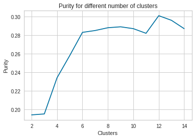
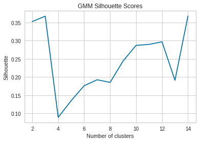
We know that the canonical number of genres in the GTZAN dataset is 10. Any result above this number is likely the cause of overfitting. The silhouette coefficient suggests that the optimal number of clusters is indeed 10, the number of genres.

However, the purity score tells a different story. For all the numbers we tested, the purity is low, which implies that this unsupervised clustering is not a good way to identify different genres. This suggests that tracks of a single genre do not necessarily share many features in common. To find a track which closely resembles an input track, it may be necessary to look in other genres.

For the transformed data GMM output, we received:

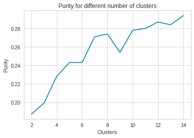
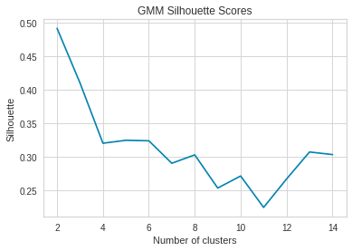
Again, the silhouette coefficient suggests that either 8 or 10 is the optimal number of clusters, but the purity score also seems to confirm, albeit with a low score, that 10 is indeed the optimal number of clusters. There was a noticeable deviation between the model’s performance on the PCA-transformed data and the original data. With both purity and silhouette coefficient scores, we hypothesize that this was due to the simplification of the data. Since so many features were removed, the boundaries between different classes were more malleable and may have blended closer together, increasing the ambiguity in the clustering and decreasing the scores of the models compared to the original features.

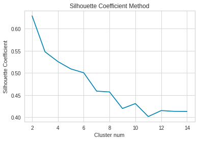
For the KMeans clustering approach, we plotted the silhouette coefficient for both the non-transformed data and the transformed data to validate our result of 5 clusters as determined by the elbow method.

Pre-transformed, original data:

Transformed Data, post PCA:

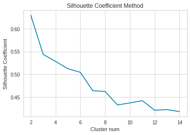
Using the Silhouette method to validate the results of the analysis was slightly less favorable. Typically, Silhouette values closer to 1 indicate less ambiguity when making decisions using a clustering algorithm, since a higher value on the scale of [-1, 1] indicates less ambiguity in terms of classifying points and more decisiveness by the algorithm, while lower values are a sign of potential conflict for data points, as they more closely to the line to the decision boundaries in the clustering algorithm. As we increase the number of clusters, we can see that the scores slightly decrease, from a high of around 0.6 towards < 0.5 with a higher number of clusters. This can partially be attributed to the increasing granularity of clusters (i.e. as the number increases, more data points fall into conflict between being part of one cluster or another, since decision boundaries are tighter, therefore increasing the Silhouette value).

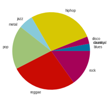
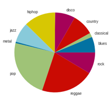
Although the silhouette coefficient didn’t fully support our optimal number of clusters as determined by the elbow approach, we decided to go with 5 as the optimal number of clusters due to the elbow approach. We have also included a visual breakdown of what each of these clusters are composed of. Original, pre-transformed data K-Means:

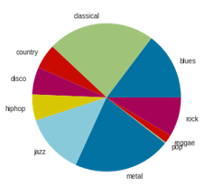
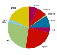
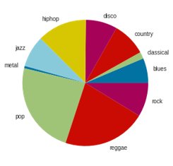
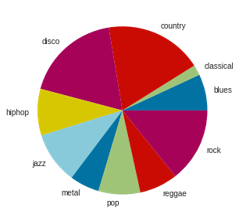
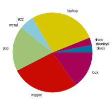
As can be seen, a cluster number of 5 does group similar genres, such as classical & blues and pop, hip hop, & reggae together.

Now, we will run K-Means on the transformed data, post PCA:

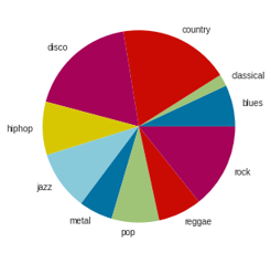
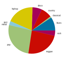
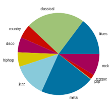
In the post-transformed feature set, KMeans seems to give some interesting results such as grouping classical and metal together. It does a good job grouping similar genres such as pop, hip hop, and reggae together. It also understandably groups classical and blues together, but also strangely groups country and disco together. It is possible that instead of grouping genres together it is actually grouping certain structures of songs together.

We also ran the purity score for the custom genres as mentioned in the results section. Purity score for K-Means with 5 components: 0.521. This means that using the custom genres did not significantly improve purity. This suggests that the genres do not form strong clusters when visualized in feature space. We also used these custom genres with supervised learning approaches.

Supervised Learning Approaches

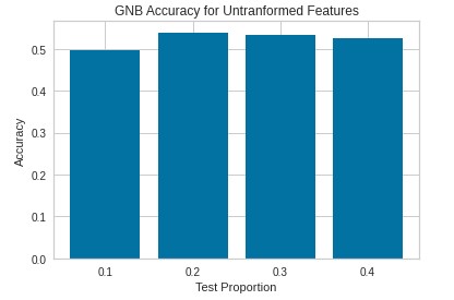
We utilized three different supervised approaches: Gaussian Naive Bayes, Random Forest, Neural Networks. Our first of three supervised learning approaches was Gaussian Naive Bayes. The first test we did utilized untransformed features and the results were as follows.

We then tried post transformed features and the results are as follows.

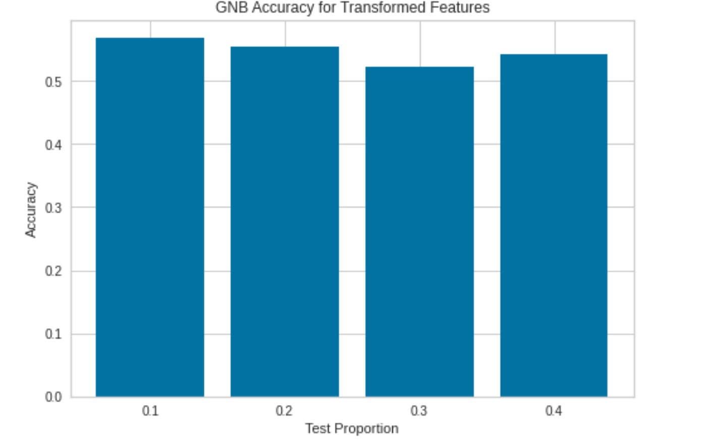
As we can see for the above graphs, on our untransformed dataset we get on average just over 50% accuracy. This is quite a decent amount as we are picking out of a large number of genres and music within genres can be quite different as seen by our earlier analysis.

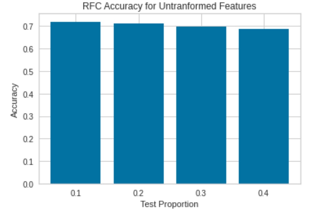
Random Forest Classifier: For the second of the three supervised learning approaches, we used a random forest classifier. The first test we did utilized untransformed features and the results were as follows:

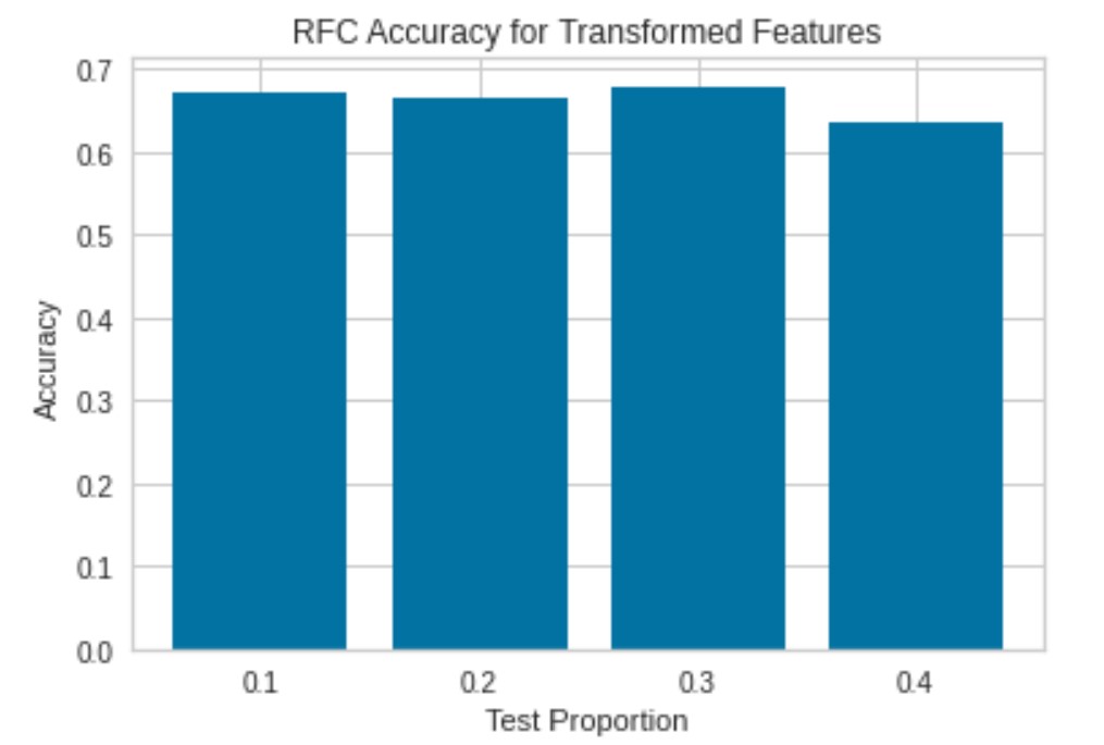
We then tried using the post transformation features and the results were as follows:

We then tried using a set of 20 different transformed features and the results were as follows:

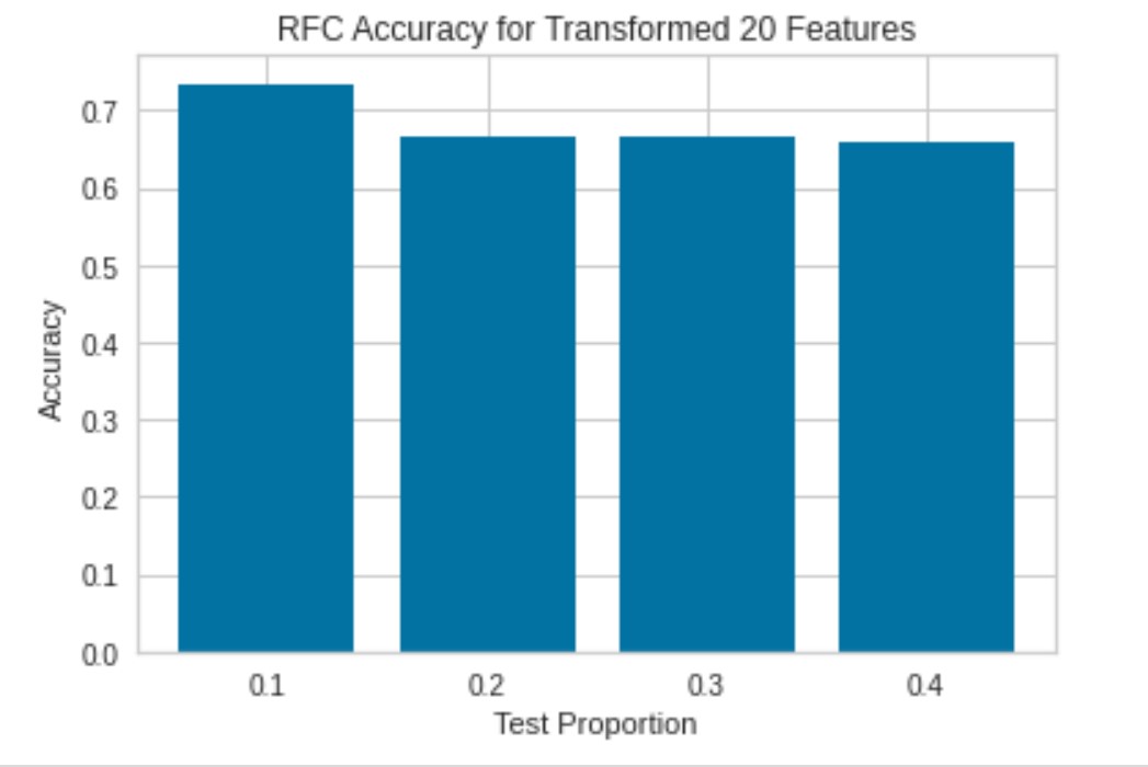
Here, we can see that RF provides a significantly higher accuracy of close to 70% on our original, which is better than our Gaussian Naive Bayes Classifier.

We also figured out the best features from this Random Forest Classifier which was as follows:

Index(['chroma_stft_mean', 'chroma_stft_var', 'rms_mean', 'rms_var',
       'spectral_centroid_var', 'spectral_bandwidth_mean', 'rolloff_mean',
       'perceptr_var', 'mfcc4_mean', 'mfcc5_var'],
      dtype='object')

Neural Networks: For the third and final approach of our supervised learning approaches, we used neural networks (NN). For our NN model, our parameters were as follows:

model = k.models.Sequential([
	k.layers.Dense(1024, activation='elu', input_shape=(features.shape[1],)),
	k.layers.Dropout(0.5),
	k.layers.BatchNormalization(), 
	k.layers.Dense(256, activation='tanh'),
	k.layers.Dropout(0.5),
	k.layers.BatchNormalization(),
	k.layers.Dense(64, activation='relu'),
	k.layers.Dropout(0.5),
	k.layers.BatchNormalization(),
	k.layers.Dense(10, activation='softmax')
])

We achieve a test accuracy of .725. This is pretty good for a difficult multiclassification problem.

Custom Genres

Below are the results for using custom genres on some of our supervised learning approaches.

categories = [
['classical', 'jazz'],
['hiphop', 'pop'],
['country', 'blues'],
['metal'],
['rock', 'disco', 'reggae']
]

We tried using our supervised learning approaches on new, custom genres. We tried fitting both Gaussisan Naive Bayes and Random Forest. We used a .80 train to .20 test ratio across all of our models to keep it consistent.

For our GNB classifier using the new labels mentioned above our accuracy was .650. We saw a slight improvement in terms of the accuracy achieved by a Gaussian Naive Bayes classifier by replacing the old labels with the new genres.

For Random Forest model with the new labels mentioned above our accuracy was .80. We again saw a slight improvement in terms of the accuracy achieved by the Random Forest Classifier by replacing the old labels with the new genres. Therefore, this assignment of genres has been shown to be a reasonable grouping of genres. We saw improvements in both models thus the assignments of genres likely make sense.

Recommendations

We recommend songs from our database based on cosine similarity (based on the features used in the random forest) to an input song. One of the results was as follows: 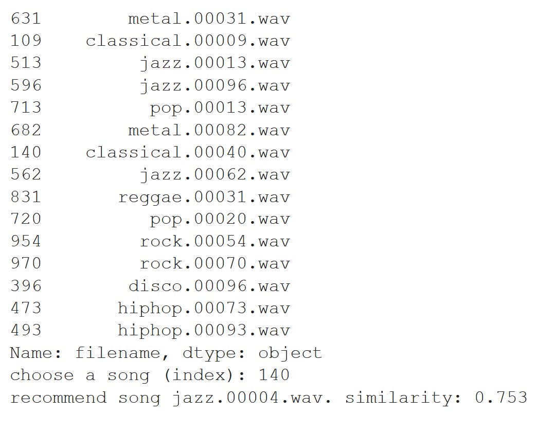As you can see, we inputted song 140, or classical.00040.wav, and it outputted jazz.00004.wav as the most similar song. As you can see this is pretty good as classical and jazz do have similarities. Recommend a song that is most different from the selected song. 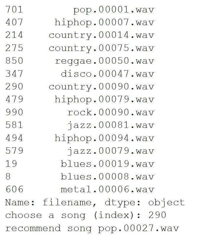As you can see, we inputted song 290, or country.00090.wv, and it outputted pop.00027.wav as the most different song. Given the type of music in these two genres, it makes sense that these songs were predicted to be different. As you can see this is pretty good as country and pop are quite different musically.

Discussion

Through this project, we successfully collected the data, transformed the data using PCA, and completed our unsupervised learning approaches of GMM and K-Means and evaluated the results. We also took a look at supervised learning approaches of Gaussian Naive Bayes, Random Forest, and Neural Networks. We evaluated those results as well. We then delved into custom genres and their potential effects on our models. We noticed that our custom genres do not have a significant effect on our models. We have also delved deeply into the features themselves to find similarities using heatmaps of correlations between the features. We have noticed some differences in KMeans and GMM and analyzed them such as the optimal number of clusters between the two. We then developed a recommendation system that allows a user to input a song and finds the most similar song using our models. Similarly, we developed a recommendation system that allows a user to input a song and find the song that is most distinct from the inputted song using our models. By doing this project, we hope strengthened our understanding of both supervised and unsupervised learning along with a deeper understanding of similarities and dissimilarities between musical pieces. In terms of difficulties with our project, two of the most difficult aspects was hyperparameter tuning our NN and effectively using SKLearn libraries. Our goal with this project successfully made it easier to categorize music and group music effectively, but our overall aim and future goal was to utilize this in a way so that users can get quality music recommendations based on the specific types of songs they like. From our analysis, most modern music recommendation tools are based on surface level comparisons like the artist rather than actually looking into the audio features of sounds, so our research is useful for creating a more powerful recommendation system.

Conclusion

Overall, through this project we were able to create effective systems for music grouping, music classification, and music recommendations, which is what we had initially intended to do. In both our unsupervised and supervised learning, we were able to get relatively good results that were verifyable and logically sound. From our results, we determined that KMeans is optimal with 6 clusters, which was about the number of genres in our dataset. We also determined that both KMeans and GMM are relatively accurate in their clustering though there is a tangible bias towards overfitted data. Then, we looked into supervised learning. We saw that Naive Bayes has a decent accuracy, though it has shortcomings because of being reliant on feature independence, which is difficult to ensure and unprobable. We also saw that RF with bagging is an extremely effective method of labelling our data with very high accuracy. Finally, we ran and tuned a NN on our data and determined that a NN is also an effective approach towards supervised learning of our data with one of the highest accuracies. After completing our supervised learning, we delved into the realm of synthetic-labels based on what we had learned in our earlier clustering. Using these synthetic-labels of metagenres were were able to record higher accuracy, highlighting the fact that metagenre utilization is beneficial to msuci classification effectiveness. Finally, we were able to apply our conclusions to a working product by extracting the most valuable features from our RF and using cosine similarity to give recommedations with high accuracy (measured by similarity and verified by inspection). Overall, we learned that for grouping music, KMeans and GMM are both effective, and for classifying music, Random Forest with bagging and synthetic-labelling is the most effective supervised approach. We also learned that for our particular data, synthetic-labelling was quite effective whereas PCA was not as effective.

Contributions

Pranay Agrawal: PCA, Elbow Method, KMeans, GMM, NN, Synthetic Genres, Recommendation

Sidhesh Desai: Elbow Method, SC, KMeans, GMM, GNB, RFC, NN

Pranal Madria: Feature analysis/ visualization, PCA, GMM, NN, Documentation/Video

Ayush Nene: Purity Score, Elbow Method, KMeans, GMM, NN, Synthetic Genres, Recommendation

Manoj Niverthi: Feature analysis/ visualization, PCA, GMM, NN, Documentation/Video

Almost all of our methods were contributed to by all of the members, the above list primarily indicates what portions each member focused on.

References

Changsheng Xu, N. C. Maddage, Xi Shao, Fang Cao and Qi Tian, “Musical genre classification using support vector machines,” 2003 IEEE International Conference on Acoustics, Speech, and Signal Processing, 2003. Proceedings. (ICASSP ‘03)., Hong Kong, China, 2003, pp. V-429, doi: 10.1109/ICASSP.2003.1199998.

D. Kim, K. Kim, K. Park, J. Lee and K. M. Lee, “A music recommendation system with a dynamic k-means clustering algorithm,” Sixth International Conference on Machine Learning and Applications (ICMLA 2007), Cincinnati, OH, USA, 2007, pp. 399-403, doi: 10.1109/ICMLA.2007.97.

Lidy, Thomas & Rauber, Andreas. (2005). Evaluation of Feature Extractors and Psycho-Acoustic Transformations for Music Genre Classification.. 34-41.

Olteanu, A. (2020, March 24). GTZAN dataset - music genre classification. Retrieved from https://www.kaggle.com/andradaolteanu/gtzan-dataset-music-genre-classification

Thierry Bertin-Mahieux, Daniel P.W. Ellis, Brian Whitman, and Paul Lamere. The Million Song Dataset. In Proceedings of the 12th International Society for Music Information Retrieval Conference (ISMIR 2011), 2011.